
Optimizing Outfielder Positioning with Limited Statcast Data
In recent years, teams have been able to leverage Statcast data to develop highly sophisticated defensive positioning models. Can I do the same with much less data?
An underappreciated innovation in recent baseball analytics has been the focus on defensive positioning. While the infield shift and its subsequent ban garnered many headlines, outfield positioning may have had a larger impact on the game. As Russell Carleton frequently discussed at Baseball Prospectus, the percentage of fly balls and line drives being caught has increased substantially the past decade bringing batting average down with it. The models fueling these positioning decisions are presumably quite complex factoring in fielder abilities, hitter/pitcher tendencies, and ballpark features. Unfortunately, much of the defensive play-by-play data being used to train these models is not publicly available. In this article, I attempt to utilize the limited publicly available data to recreate a basic outfielder positioning model. The goal of this project is to explore the process required to build these models while also discussing challenges and workarounds of modeling with incomplete data.
Specifically, I do the following:
· Reconstruct an approximate dataset of outfielder defensive opportunities utilizing visualizations provided by Baseball Savant
· Develop Machine Learning models to predict individual defender’s ranges using small and imbalanced datasets
· Build a model of Wrigley Field run values highlighting regions which are more critical for defensive coverage
· Propose a loss function to optimize outfielder positioning with the goal of minimizing potential offense
Problem Overview
The goal of this project is to build a Machine Learning model which finds the optimal defensive positioning for a group of outfielders in a specific ballpark. I hope to use this project to gain experience building my own defensive models and demonstrate my process of how I approach a complex task. For the sake of this project, I elected to focus on Wrigley Field and the Cubs starting outfield of Ian Happ, Pete Crow-Armstrong, and Kyle Tucker. This choice was arbitrary and this analysis could be replicated with any set of players and stadium.
My final model is composed of three different steps. In step 1, I model a player’s range and predict the probability they will be able to catch a fly ball based on the location relative to their starting position. Next, I attempt to measure how costly it is to allow a given fly ball to fall for a base hit by predicting the run value of a base hit’s location. Finally, I search for the outfielders’ positions so that their ranges cover the maximum total run values (or minimize the total uncovered run values) in the field of play. The key idea being that a ball landing for a double is costlier to a team than a single and, all else being equal, the outfielders should protect against the double more than the single. However, if covering the double leaves too much area uncovered this will result in too many singles offsetting the gains. The goal is to find the optimal point to balance this trade-off.
What makes this project especially interesting to me is the lack of available data. While Baseball Savant publishes aggregate fielding data at a team and player level, most of the play-by-play data is restricted. Fortunately, even with the data they do provide, standard computer vision techniques can be applied to reconstruct a small dataset to serve as the foundation of the models.
Throughout this project, I make several simplifying assumptions which would theoretically limit the final’s model utility in practice. I detail these assumptions as they arise. While teams already have rather sophisticated models in place tackling this problem, they also have access to much more data. Despite these limitations, I believe the final model is representative of a first attempt which could be iterated on in production. My objective is to focus on the process and how to overcome some of the unique challenges in this problem.
Data
All data in this article is sourced from Baseball Savant. I downloaded Statcast data for balls in play at Wrigley Field between 2020 and 2025. This includes information such as hit locations, launch speed and angle, and event type.
Unfortunately, there are several limitations to this data for my purposes. First, the hit locations are stored in variables named hc_x and hc_y, but from the documentation it is unclear exactly what these locations represent. For example, I am unsure what the scale of these attributes is because they do not map to feet. The data also does not include definitions for the location of home plate. Neither of these are prohibitive to my goals but they do complicate the analysis slightly.
More importantly, the data does not include any information regarding defender positioning either before or during the play excluding both distance to ball and catch probability. Instead, the player pages include a chart of all “responsible plays” for a fielder. For example, the below chart for PCA illustrates all the balls in play which were hits or outs as well as his typical starting position:
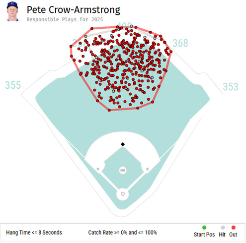
Again, this data has its own limitations. It is unclear how a player is assigned a “responsible play”. For example, if a sharp line drive is hit to right center field where neither player has a reasonable chance of catching it, is it assigned to the center fielder, the right fielder, or neither player? Based on my observations, it appears this would be assigned to neither but I could be mistaken. Furthermore, I am unsure how the starting position for each player is decided (i.e. is it an average, median, or modal starting position). It also seems that batted balls are marked based on their true location regardless of where the fielder was positioned. This would suggest that if a fielder is in a heavy shift, a ball could land far from their current location but very near to the graphic’s start position providing a misleading representation of the difficulty of the play. While accessible by hovering on the browser, the downloaded charts also do not include hang time or catch probability further obfuscating the difficulty of a given play.
Despite these challenges, these charts effectively provide a general overview of a player’s range and their success rate, the details needed for predicting a defender’s range. I downloaded the charts for each of the Cubs starting outfielders as of August 15, 2025.
Outfielder Range
The simplest version of a model for an outfielder’s range requires two features: distance from and direction towards the ball in play. Distance is the more obvious of these. A player is only able to cover a certain amount of ground based on factors such as their speed and reaction time. Naturally, a ball hit directly at a fielder should be easier to catch than a ball hit 200 feet away. The direction towards the ball, however, is equally relevant. Fielders will naturally be able to cover more ground in some directions than others. For example, running backwards is generally more difficult than running forward because the fielder must turn around while tracking the ball over their shoulder. In theory, a fielder’s range is expected to be larger in front of them than behind them, but this dynamic could apply to running other directions as well.
While this data is not provided directly, it can be inferred from the graphics on the Baseball Savant player pages. The above image displays PCA’s typical starting location, his hits allowed, and balls fielded. Using tools from computer vision, the locations of each of these points can be identified in the image and their relative location measured.
Building the Dataset
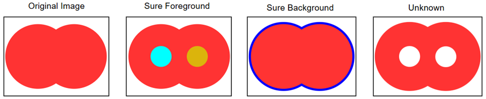
The watershed algorithm can be used to detect individual, overlapping shapes in an image. To run this, I first must clean the image by creating a mask which identifies all the pixels of a particular color (e.g. red for outs) and removing all other details from the image. Then, I divide the image into 3 areas. First, the “sure foreground” is the part of the image that certainly belongs to a point in the original picture. This is calculated by measuring the distance of each pixel in the group to the nearest pixel outside of it. Pixels with higher distances are likely to be close to the center of an individual point. Next, I need to figure out the “sure background”. These are pixels which positively do not belong to a point. This is calculated with a dilation transformation which increases the size of each point. Finally, the unknown region is measured by taking the difference between these. This procedure is demonstrated in the following image:
The watershed algorithm imagines the image as a topographic map where a pixel’s height is measured by the distances calculated earlier. In this mapping, the sure foreground pixels form basins. Imagine filling the basins with water. As they flood, the unknown pixels become covered and get assigned to their respective foreground groups. The water levels continue to rise until the two basins intersect. The connection pixels form the boundary. Once the entire image is fully flooded, every pixel has been assigned to a group and we can distinguish between the two overlapping points. I’ve created the below gif to demonstrate the general idea in practice.
With this algorithm in place, let’s revisit the graphic showing PCA’s responsible plays. I have taken the original graphic minus the convex hulls and placed a blue dot on every hit and a yellow dot on every out. While difficult to see, there is also a green dot indicating his starting position. The watershed algorithm generally does a good job of separating individual points. While there are some misses and some clusters that are recognized as a single point, there is enough data to approximate the location of the balls in play assigned to PCA.
I repeated this process for both Tucker and Happ to generate similar plots for both of them. I then scaled each of these observed points to correspond to the actual x, y coordinates in the field of play. Next for every ball in play, I calculated the Euclidean distance and angle in radians from the fielder’s starting point to the ball’s location. These are the features I used to build the dataset for each player.
Modeling Outfielder Range
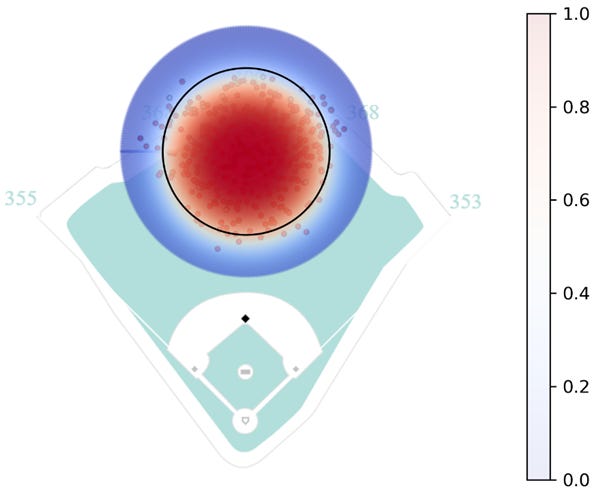
To predict a fielder’s range, I would like to use a logistic regression model with features for distance and angle. However, because the angle is not a linear feature (i.e. 0 and 2π are equivalent despite appearing as two opposite extremes), the angle needs to be embedded as its x and y components by taking the cosine and sine, respectively1. As a first pass, I fit a model for PCA using these features where the target variable is whether the ball is an out or hit. Below is a heatmap showing his predicted range.
Clearly, this model has problems. According to this heatmap, PCA has at least an 87.5% chance of catching any ball that is hit within 150 feet of him. This is obviously incorrect, so what happened?
The answer is simply that the data is biased. In my last post, I discussed the issue of imbalanced learning, and it reappears here. Looking at the figure from above, almost all of the batted balls assigned to PCA are caught for outs, 93% to be precise. The model sees almost all outs and in turn predicts almost all outs, but in this case identifying those hits are more important.
Another issue here which also contributes to the imbalance is the definition of “responsible plays”. Batted balls are not assigned to PCA unless he has some reasonable chance of catching it. Think of a ball hit down the left field line. Practically speaking PCA has no chance of catching it and as such he shouldn’t be punished with a hit against his record. Unfortunately, by removing it from the data, the model does not have a chance to learn this fact. It needs to see which balls he did not make a play on in order to define the limits of his range.
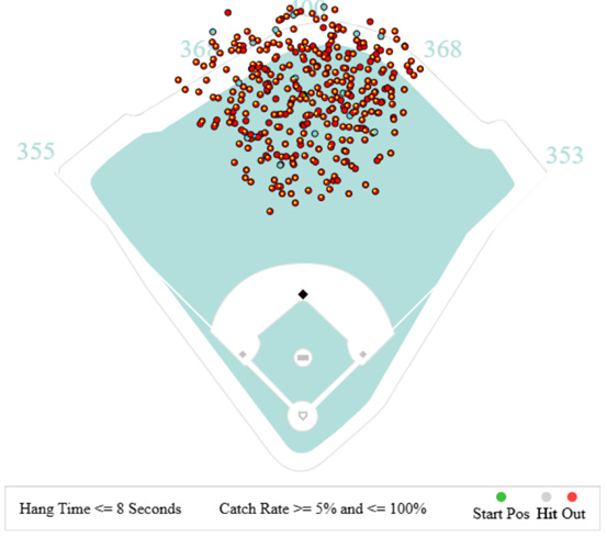
Fortunately, I already have access to many balls in play which PCA did not make a play on. Specifically, any ball that was caught by Happ or Tucker is a ball that was not caught by PCA. While this assumption is imperfect2, it provides a good enough estimate. Adding these points to the dataset and the new map of responsible plays looks like this:
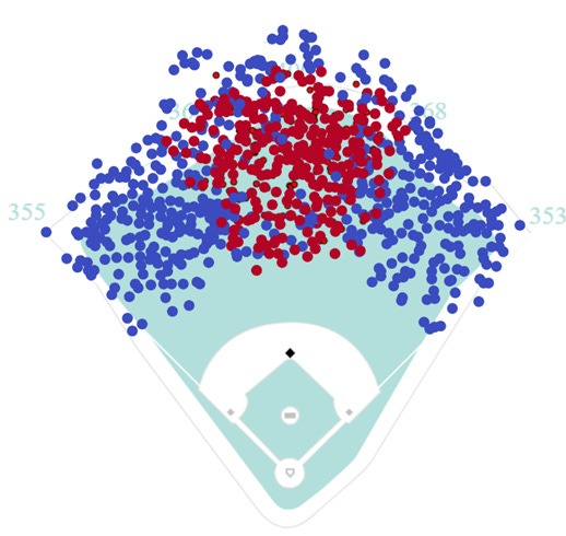
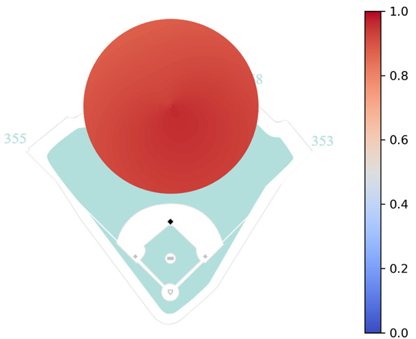
Clearly, this data provides much better coverage of the outfield and more truly represents PCA’s range. Retraining the Logistic Regression model from above with the new data returns the following heatmap:
This output looks much better. The point where the catch probability crosses the 50% threshold on average occurs at a distance of about 100 feet. There are a few actual outs in the low probability ranges consistent with the idea that these plays are possible but rare, and balls more than 150 feet away have a catch probability of only a few percentage points. Additionally, the heatmap is slightly skewed showing that direction does make a difference on catch probability. Specifically, batted balls in front of PCA have a higher catch probability than batted balls behind him at equal distances, consistent with intuition.
This model is surely imperfect. It could be expanded to account for features such as hang time, launch angle, or launch speed to provide a more sophisticated representation. But based on the provided evidence, this appears to be a worthwhile approximation of PCA’s range. I repeated this process to create similar ranges for both Happ and Tucker.
Stadium Run Values
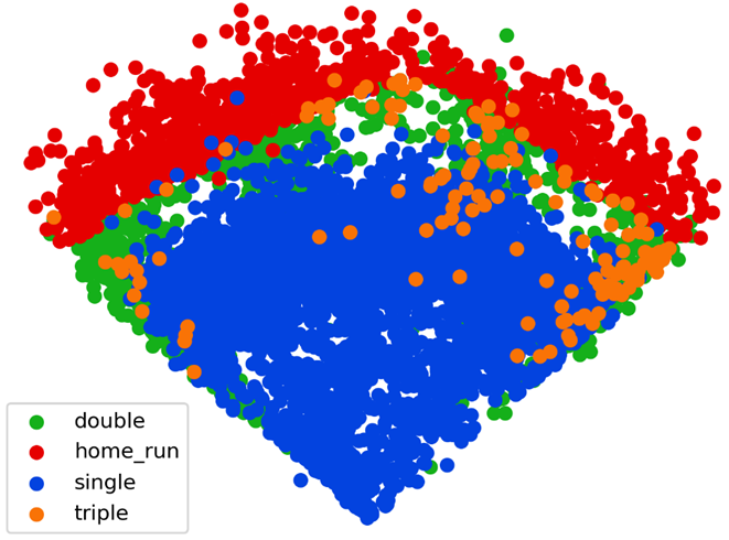
Now that I estimated individual fielder’s ranges, the next step is to figure out the areas of the field which are most important for them to cover. In order to do this, it is necessary to calculate the run value of a ball in play based on its location. The below image shows all base hits at Wrigley Field from 2020-2025.
However, there’s an issue with this data. As mentioned above, the data used to generate these plots are stored in variables called hc_x and hc_y. At this point, it is unclear to me what units these features are in but they are not feet. This will be a problem later on when it is time to match player’s ranges to these run values. To prevent this, it is necessary to transform these unknown coordinates into the same scale as above3.
The data from Baseball Savant includes hit distance. On groundballs and base hits, the ball rolls prior to being touched and it is unclear how this distance feature matches up with hc_x and hc_y. However, for flyouts, popouts, and lineouts, these data theoretically should be a perfect match to the distance from home plate. Assuming a linear transformation from hc_x and hc_y into feet, it is possible to compare the actual distance in the data against the calculated distances from home plate to estimate the scalar value. Note that the location of home plate is also unknown in the data and needs to be estimated. Unfortunately, there is no one set of values that perfectly aligns with all the data, so these parameters need to be estimated.
I defined the following loss function which measures the mean squared error between the projected batted ball distance and actual batted ball distance dependent on parameters hpx, hpy and α where hpx and hpy are the x and y location of home plate, α is a constant, and Di is the actual distance of the batted ball.
Using scipy, I was able to find the parameters which minimized this loss function across all outs. The resulting home plate coordinates were (126.2, 210.2) with an α of 2.28. Others have previously attempted this problem and reached similar coordinates for home plate. Further, the projected distances match the actual distances with an R2 of .96 suggesting a strong correlation.
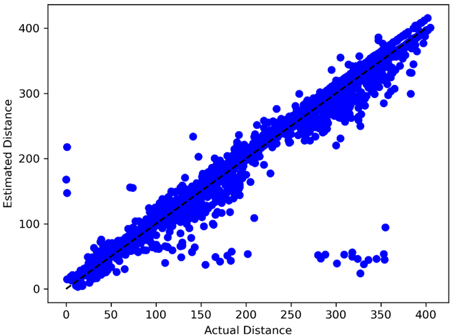
Given this, I am confident that these projected parameters are a faithful representation of the true values. Applying this transformation to the data, I can now map the base hits from above against an outline of Wrigley Field.
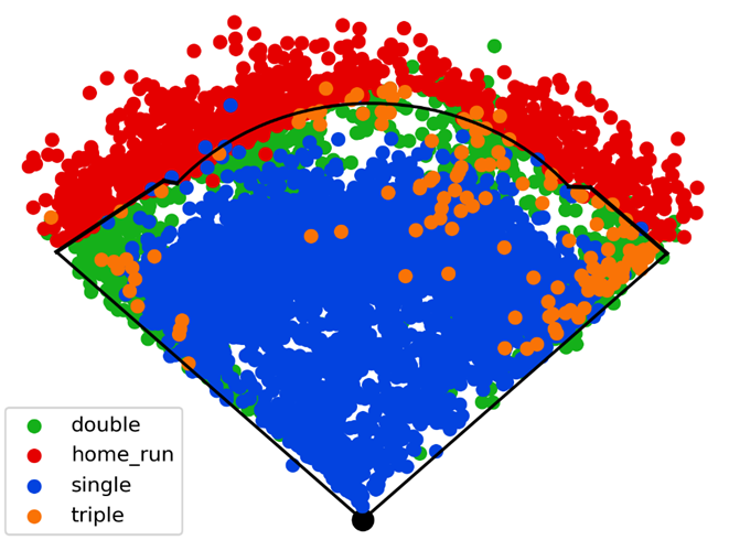
I simplified the outfield walls to make the math easier in the next steps. Specifically, the wall in left center should be a little straighter and shallower while the area just to the right of center should be deeper. Other than that, this visual again appears faithful to the actual data. The hits run up against the foul line but rarely cross over it, and the outfield wall generally does a good job of separating home runs from balls in play.
The next step is to predict the run value of a ball in play based on its location. For the uninitiated, run values are linear weights that attempt to measure the relative contribution of a hit. For example, in slugging percentage a single is worth 1 point while a home run is worth 4, but it is not necessarily true that a home run is 4x more valuable than a single. In fact, when we do the math home runs are actually about 2.3x more valuable than singles. The exact run values vary year to year and are available on Fangraphs.
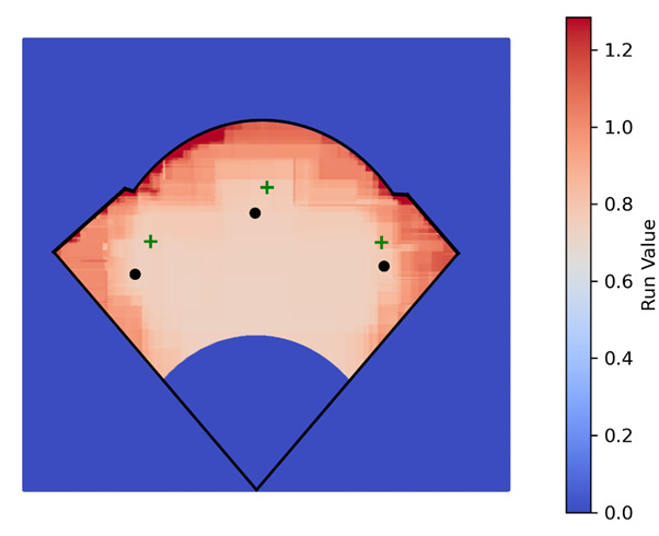
I converted the base hits into their respective run values and fit a regression model to predict the run value of a base hit dependent on its location. There are a few limitations to this approach. Specifically, I assume that the run value is the same no matter who is running the bases or where the fielder is positioned, both of which are unrealistic, but as has been the theme throughout this article, it should be a good enough approximation. Using XGBoost, I predicted the run value of all batted ball locations. Because the end goal is to use this for outfield defensive positioning, I manually adjusted all run values in the infield, foul territory, and beyond the fences to 0. The result looked like this:
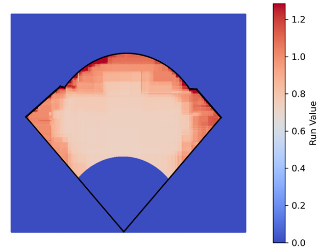
Again, the results are consistent with intuition. Balls hit shallow and in the middle of the field typically go for singles while hits down the line and to the corners are more likely to go for extra bases. Finally, this output can be combined with the individual fielder models to optimize their positioning.
Optimizing Positioning
Ideally, the goal of defensive positioning is to prevent more costly extra base hits to the best of our ability. However, there is an inherent trade-off that by covering areas which are more likely to go for doubles or triples, fielders are allowing more room for singles. As such, the goal for the outfielders should be to leave the minimum total run value uncovered.
This target can be formulated as a loss function:
The probability that an individual player catches a ball at point x,y is represented by the function p(x,y) while the run value of the point is the function r(x,y). The functions for p vary based on the starting position of the fielders. At each point, the probability that a ball is not going to be caught is multiplied by the run value if the ball is not caught. The sum is then taken across all points. For balls hit in between fielders with overlapping ranges, I chose to assign it to the player with the maximum probability of catching the ball. A more sophisticated approach could handle the dependencies between catch probabilities, but this should suffice for these purposes. Using scipy, I found the positioning of the three fielders that minimizes this loss function.
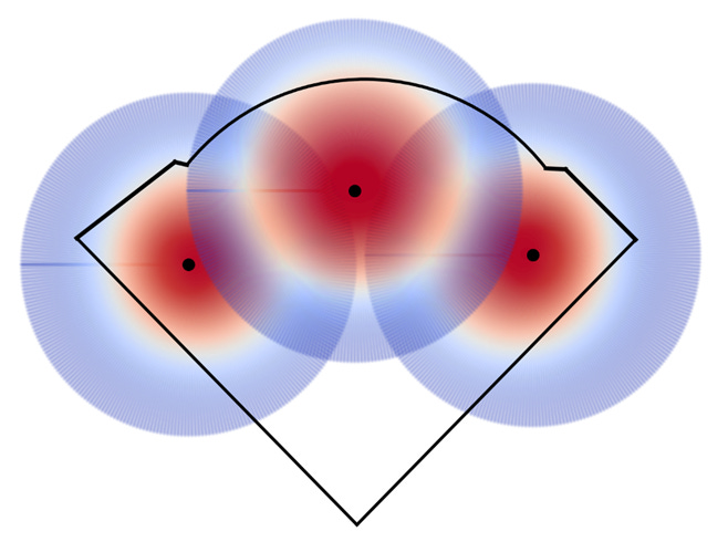
At first glance, this looks like normal outfield positioning. PCA has a large range in center so Tucker and Happ are positioned slightly towards the lines to make up for that fact. Speculatively, better estimates for the probabilities of catching balls hit to the alleys might indicate that the corner outfielders should pinch towards the center to better cover those areas. While not present in this model, Wrigley famously has almost no foul ground in the corners so there’s even less of a need to cover that territory.
Comparing the predicted locations to the actual ones there are some key differences. Namely, as already discussed the corner outfielders are guarding the lines slightly more than the actual players. However, the actual players also start further back than predicted. This could be due to a number of factors. First, I did not model the infielders. Instead I cut the infield off at the dirt. In real life, the second baseman and shortstop will be able to cover some of the territory that the model is assigning to the outfielders, especially when those players are gold glovers like Dansby Swanson and Nico Hoerner. Additionally, it could be possible that the model is underestimating the difficulty of catching balls against the wall or the difference in running forward versus backwards. Both of these could bias the model to moving fielders too far in. In the below table I show each player’s projected starting position against their actual position according to Baseball Savant4:
All things considered, I think these estimates are pretty good. As discussed at length, there are many minor improvements to make each of which will push the model closer towards an optimal solution. However, it is clear why the model is behaving the way it is and where the biases are entering. Overall, this approach appears to be a strong foundation which a team could iterate on in practice to develop a functioning positioning model.
Conclusion
When I dreamed up this project, I envisioned a quick and easy 1500-word post detailing a defensive positioning model. Nearly 4000 words later, this project has been anything but that. However, that’s also what made this so much fun to work on.
Throughout the process, I experienced a number of issues which are common in real-world applications. The reality is that much of the data teams rely on for these models are not publicly available. This lack of public data required some creativity in recreating my own dataset. The result was not a perfect representation of real-world data, but nonetheless had enough utility to accomplish the task. I also encountered another imbalanced learning problem and discussed the importance of having reliable, quality data for modeling. Working through these issues and training my problem-solving skills are the reason I enjoy these projects as much as I do.
As I stated at the beginning, my goal was not to build a final production-worthy model, but to work through the process and develop the foundations of a model which could be iterated on in practice. This approach definitely is not optimal. There are many limitations and each one drifts the model further away from a practical application. On the other hand, at every step, I checked the output of the model against real world data and my own intuition, and while the results are imperfect, they generally match pretty well. Ultimately, the end results demonstrate that we are able to develop our own working version of a model which serves as a decent proxy for an in-production model despite the limitations.
I elected to do it this way to preserve distance as its own unique feature while avoiding dependency between features. A simpler approach using Δx and Δy as features directly would be viable as well.
PCA may not have played that night; the ball could have been catchable by both players but PCA deferred to his teammate; etc.
1 pixel:1 foot
For reference, home plate is at (288, 0)