
Exploring Imbalanced Learning in Projecting Starting Pitcher Performance
Imbalanced learning is fundamental to model development but how is it something we can use to improve baseball analysis?
A fundamental challenge in Machine Learning (ML) is imbalanced learning. Effectively recognizing and addressing imbalance is an essential step in developing high-quality models. Unfortunately, it frequently does not get the attention it deserves in the public sphere, especially in baseball research. In this article, I demonstrate the importance of considering imbalance when analyzing ML models and explore its application in a classic baseball setting. Specifically, I contribute the following:
Detailed background on the problem of imbalanced learning and examples as to how it pertains to baseball;
Step-by-step walkthrough of development of a simple predictive model to project starting pitcher performance as measured by FIP- while exploring concepts such as time series forecasting, feature selection, data standardization, and small sample size;
Demonstration of how to restructure the optimization problem from step 2 through the lens of imbalance;
Analysis of the models from steps 2-3 including a robust discussion surrounding the strengths and weaknesses of such an approach.
Imbalanced Learning Background
Imagine you were presented with the details of a random credit card transaction and were asked to identify whether or not it was fraudulent. The amount of fraud is somewhere around 0.1% of all credit card transactions. Given this fact, with no other information or expertise, you would probably predict the transaction is legitimate, and 99.9% of the time you would be correct. This naïve model that always assumes a transaction is legitimate has an extremely high accuracy, but it is also useless in practice. The real value of such a model is being able to identify the fraudulent transactions when they do occur.
This scenario is an example of the imbalanced learning problem, and it is a fundamental issue in Machine Learning. Imbalance refers to a situation where data is disproportionately distributed in such a way that causes a skewed representation of critical patterns or concepts within the data. In the above example, the data is heavily skewed towards legitimate transactions making it more difficult to identify the critical patterns that indicate fraud. Other classic examples of imbalanced problems include email spam detection, rare disease diagnosis, or defect detection in manufacturing. A commonality across all these domains is that one value is far more important to predict accurately than the others. Our model from above has 99.9% accuracy overall but 0.0% accuracy on the important, fraudulent cases.
Unfortunately, the issue of imbalance is too often overlooked in ML. Much of the literature in this space is focused on data imbalance, that is situations where an individual class is over-represented in the data (as in the above example). When not careful, this can lead to undesirable behavior where a model always outputs the majority class. However, the problem is more complicated than this. Characteristics such as data noise, borderline cases, and overlapping/inseparable classes all contribute to the complexities of imbalanced learning. Additionally, while we frequently focus on imbalanced learning in a classification setting where there is clear class separation, these problems persist in regression where a given range of values is more important to predict correctly than others.
While rarely discussed directly, these problems are prevalent in baseball, too. For example, assume you had projections for two different shortstops: Player A is projected to produce 2 WAR while Player B is projected for 6 WAR. Is one of these players more critical to project accurately? Let’s assume that in both cases, the projection was actually 2 wins too high. That is, the true value of these players was 0 WAR and 4 WAR, respectively. While the error is the same in absolute terms, the practical consequences may differ. If a team signed Player A, they may have wasted resources on a replacement level player, but they will probably be able to find an upgrade via the trade market or a midseason promotion. In the case of Player B, however, the team was expecting a star player but instead had to settle for above-average production. This shortfall is much more difficult to address. If they are a team on the edge of playoff contention, they may have been relying on those 2 additional wins to secure the postseason.
From a roster planning perspective, the projection error on Player B is more damaging. In this sense, it is more important to predict Player B accurately than Player A. This represents the core idea behind imbalanced learning: some outcomes matter more than others. Other baseball contexts where this could apply include prospect grading (identifying above average players is more important than recognizing an organizational filler), pitch framing evaluation (some pitch locations provide “more valuable” stolen strikes than others), or injury risk assessment (anticipating whether a player is likely to have a season-ending injury or a more minor IL stint). In each of these examples the learning tasks involve unequal costs, making them natural cases of imbalanced learning.
Problem Statement
In this project, I seek to demonstrate the benefits of approaching a standard baseball ML project with imbalanced learning. For the specific problem, I attempt to project starting pitcher performance using FIP-. Typically, this problem is addressed by trying to predict the player’s performance directly. However, I argue that the real value of such a model is to identify players who are expected to dramatically improve or worsen in the coming season, recognizing players who are more likely to be under- or over-valued. This is the imbalanced nature of the problem.
I begin by fitting a standard ML model without regards for imbalance but thinking through many of the steps we may want to consider when building a basic projection model with baseball. Once this model is in place, I repeat the process but directly optimizing for imbalance and applying more weight to predicting the players with the biggest year-to-year changes in FIP-. Finally, I will compare the best models both with and without considerations imbalance and analyze their strengths and weaknesses.
Data
Data for this project was downloaded from Fangraphs including all player seasons from 2017-2024[1] with at least 15 IP as a SP. Downloaded features included overall performance measures (e.g. FIP-, xFIP, K%), batted ball results (e.g. GB%, Hard Hit Rate, HR/FB), and plate discipline statistics (e.g. O-Swing%, Z-Contact%). The goal is to use this data to predict a player’s FIP- in the upcoming season.
This is a time series forecasting task. To provide the model with as much context as possible, we want to combine player’s past performance over multiple seasons to predict the next season’s performance. In this case, I elected to use a rolling window of two prior seasons to train my model. That is, data from the 2022-2023 seasons were used to predict 2024 and 2021-2022 data to predict 2023, etc. Players who did not reach the IP threshold in three consecutive seasons were removed from the data. This left 578 players in between 2019-2023 seasons who were used as train data and 117 in 2024 for the test data.
Before we begin, I want to highlight a key limitation of this dataset which I am considering beyond the scope of this article. By removing all players who fail to reach the IP threshold as a SP, I am introducing a survivorship bias into my data. Better players are inherently more likely to reach the threshold and will therefore make up a larger proportion of the dataset potentially biasing the model. Not considering survivorship bias limits the real-world utility of this project but should not hinder my ultimate goal of exploring the issue of imbalance. I may come back to this in a future project because I think it is an interesting topic on its own but not within this context.
Model Development
To begin, its necessary to establish a baseline performance that we can use as a point of comparison. In this case, my baseline is to assume that a player will perform identically in year X as they did in year X-1. That is our prediction for a player’s FIP- in 2024 is simply their FIP- in 2023. Any model which fails to outperform this bare minimum standard offers no value to us as forecasters. I will evaluate models using three metrics: R2, Mean Absolute Error (MAE), and Mean Squared Error (MSE).
For my experiments, I compared models using two different solutions. First, Linear Regression (LR) a simple approach that fits a linear function by minimizing the sum of squares between the prediction and the target. Because it assumes a linear relationship, LR often fails to capture more complex patterns in the data. However, it can still be useful, especially when working with smaller datasets, due to its simplicity and low risk of overfitting. Extreme Gradient Boosting (XGB), on the other hand, is a more advanced and powerful method. It builds an ensemble of small decision trees where each tree learns from the mistakes of the previous ones. This process allows XGB to capture more complicated relationships in the data.
To start, I fit initial models using the train data from 2019-2023. At this stage, all features were included in model building. Here are the initial results on the 2024 test data:
Here I am using the scikit-learn implementation of R2 which is able to be negative suggesting low predictive performance. Initially, both XGB and LR outperform the baseline with LR performing best. However, there are several steps we can consider to mitigate bias and further improve this model.
Feature Selection
The current version of this model is trained on 578 samples and 30 features. Generally, it is better to use a small set of high-quality features than to include all available ones. This is especially true with Linear Regression where a higher sample-to-feature ratio reduces the risk of overfitting. Furthermore, many of the features we are currently using are either weakly correlated with the target variable or highly correlated with other features. Irrelevant features add noise, while multicollinearity can make model coefficients unstable, both of which can degrade model performance.
Instead, it is better to perform feature selection, a process by which we choose a subset of the most relevant input variables from the dataset. We then train the model solely on these features. For the purposes of this project, I used Univariate Feature Selection through the scikit-learn package in python. Specifically, I used the SelectKBest algorithm which evaluates each individual feature’s F-score with the dependent variable and then keeps the k best features. The hyperparameter k was selected through a cross-validation grid search.
Comparing the results from using feature selection to above, we can see that incorporating feature selection improves MAE in LR though with slight degradation in R2. However, combining feature selection with other techniques may further improve performance.
Standardization
Next, we want to consider the changing environments in baseball. Performances across different seasons are not directly comparable due to shifts in league-wide trends. For example, from 2014 to 2024 the league average strikeout rate increased from 20.4% to 22.6% - a change of more than 10%. Our goal is to build a model which is robust to these changes.
To address this, I standardized each of the individual features by subtracting the league average and dividing by the standard deviation for each season and statistic[2]. This transformation converts raw statistics into z-scores, measuring a player’s performance relative to the league as opposed to focusing on the absolute values which may be misleading on their own.
Combining this change with feature selection improved performance for both XGB and LR over the basic models in both R2 and MSE.
Sample Size Adjustments
Finally, we should consider the impact that small sample sizes can have on our model. A fundamental issue with baseball analysis is that many statistics do not stabilize until several hundred batters faced. However, our data consists of all player seasons with a minimum 15 IP, well before many statistics stabilize. This means that many of the features our model is currently trained on may be noisy or misleading.
To address this, we can apply regression to the mean to blend each player’s observed stats with league averages, adjusting for playing time. I used the following formula where Xi is a single sample, IPi is the number of innings pitched that player had in a season, is league average performance, and k is a hyperparameter attained through grid search:
Essentially, this formula assumes that each player’s season included an extra k innings pitched of league average performance. The model was then trained on these new values. Doing this helps to prevent outlier cases where players had exceptionally strong or weak seasons over a small sample while preserving players who had legitimate breakouts or slumps.
Applying this with feature selection improves performance in MAE against standardization with the XGB version finishing first.
At this point, we have 8 models significantly outperforming the naïve baseline. With just a few basic steps, we have been able to improve performance to such an extent that we can feel reasonably confident in the overall quality of our model. However, none of these models address the imbalanced nature of the problem.
Relevance Function
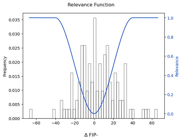
As introduced above, the main issue with the current evaluation is that it treats all FIP- values equally, but some values are more important to predict correctly than others. Specifically, we care more about larger changes in FIP-. We can represent this using a relevance function which assigns a score from 0 to 1 for different changes in FIP- values. A higher relevance score indicates that the value is more important to get right. The relevance function is typically defined by a domain expert with direct knowledge of the values on which they want to focus.
In this case, I manually assigned a change of 40 or more points in FIP- to have a maximum relevance score, and a change of 0 points to have minimum relevance. These values were chosen to illustrate the idea of imbalance, though in practice they are flexible to a team’s specific needs. This plot shows the distribution of ΔFIP- in the test data and the corresponding relevance values.
SERA
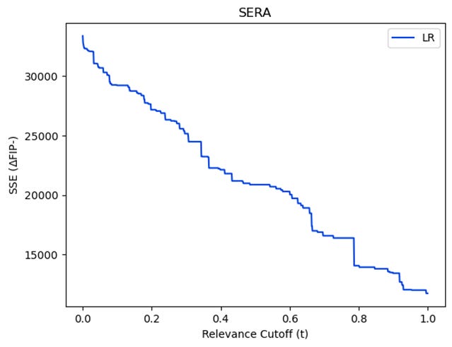
With this relevance function, we can now measure the quality of our models while explicitly considering imbalance. I have elected to use Squared-Error Relevance Area (SERA) to measure performance. SERA is an error measurement similar to MAE or MSE where a lower total is better. SERA is computed by measuring the area under the Squared-Error Relevance Curve - a plot of the sum of squared errors (SSE) for all observations with a relevance score above a given cutoff t. As t increases along the x-axis, only higher-relevance observations are included in the SSE.
Dt is the subset of cases within the dataset D that have a relevance equal to or greater than t, is the predicted result for sample i and yi sample i’s true value. Intuitively, by integrating over all values t, observations with higher relevance scores are counted multiple times effectively giving them greater weight in the final error score. This allows the measure to focus more heavily on the cases that matter most.
As an illustration, here is the Squared-Error Relevance Curve for the original LR model after adjusting the predictions to represent the change in FIP-. At a relevance cutoff of 0, the SSE is equal to the SSE across all observations. Meanwhile relevance cutoff 1 only includes players who had a ΔFIP- greater than or equal to 40, those observations we care most about. The curve is always monotonically decreasing. SERA is the area under the curve.
Now we can return to the table from above but now including SERA:
Imbalance Optimization
At the moment XGB with feature selection and standardization is the top performer in SERA. However, this model is currently being optimized using MSE. A key benefit of SERA is that we are able to use it as the loss function directly considering domain imbalance during model training.
I reran the experiments from above except this time I used XGB optimizing directly for SERA (XGBSERA). The following table shows how the new top performing models compare. Note that R2 in XGBSERA is measured using the implied FIP- from the projections for consistency.
Discussion
As expected our new models, dramatically improve upon our original models in SERA with a small cost in MAE and MSE. We can examine the SERA graphs for each of the models and the original baseline to better understand their strengths and weaknesses of each.
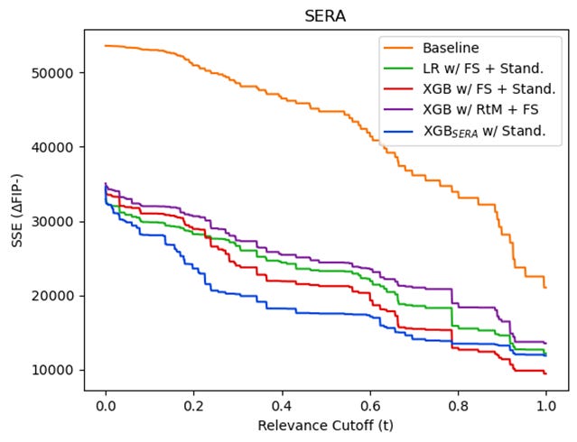
LR is the best model in terms of MAE and MSE. However, these graphs illustrate that much of its success is focused in the low relevance cases, those which we care least about predicting accurately. Our new model, on the other hand, while second-worse in MSE is the best at predicting players with relevance scores between approximately 0.05 and 0.8. Our model is much better at anticipating players whose FIP- will change by about 10-30 points, an important group for recognizing breakout or disappointing players.
We can explore this further by looking at a scatter plot of players performances in 2023 vs 2024. The size and color of the points correspond to the predicted change in performance by each model. The dashed line represents identical performance in both seasons. In a perfect model, every red point would be above the line, every blue point below the line, and the size of each point would increase as the distance from the line increased.
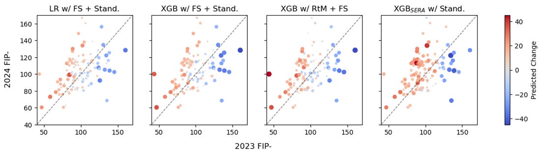
Visually, it is apparent that pitchers with relatively small but meaningful changes (i.e. ~20-30 points) are much better represented in the SERA-based plot which is consistent with our finding from above. The points in that range on the right-most plot are bigger and darker colored than each of the other plots. Even though the XGB w/ RtM + FS model is better at the most extreme outliers, it is less effective on many of the middle cases.
Every modeling decision, however, comes with trade-offs. The model optimized with SERA is more likely to predict larger movements than each of the other 3 models. The MSE-based models are somewhat conservative in predicting larger changes as evidenced by the large number of small, pale points. The SERA-based model, however, is much more aggressive and that resulted in lower R2 and higher total error. The SERA-based model has a bias against assuming players will perform the same in two consecutive years even though that is typically the starting point for most analysis. In a real-world application, an analyst would have to weigh these costs and benefits to determine which one is best for their specific problem.
Conclusion
Ultimately, the purpose of this article is to illustrate the benefits of viewing standard baseball problems through the lens of imbalanced learning. Context matters when developing ML models, and it is important to incorporate those real-world priorities into the training process. Imbalance offers a structured way to accomplish this.
There is never a single best way to design a model, and there will always be trade-offs. In this case, we saw that optimizing for SERA resulted in lower R2 and higher total error. However, if the purpose of this model was to identify which talent to target, the small differences in FIP- for an established talent might be less important than appreciating the players who the market is evaluating improperly. The key to responsible model building is not to search for a one-size-fits-all approach, but instead to make deliberate choices that align with the specific goals of the problem. Thinking about problems in terms of imbalance provides us with a better toolbox to address these issues directly, and, hopefully, can lead to more effective models.
[1] 2017 was chosen arbitrarily.
[2] For simplicity, I used the means and standard deviations observed in the dataset rather than the true values including all players across the league